March 16, 2020
For the exploratory analysis project performed, I chose to combine two datasets by the country variable. The first dataset I chose was about average plastic waste per country that was measured in kg/person/day. The first dataset was obtained from GitHub’s tidytuesday project. In addition to containing average plastic waste, the first dataset also included the country’s three letter code, the GDP per capital of each country in the data set, year, and total population of the country. I chose this dataset because I was very interested on the trend in plastic waste in countries around the world. I was hoping to compare the different countries to see how plastic waste relates to other aspects of a country such as GDP and population. The second dataset I chose was a dataset about the average life expectancy (in years) in various countries. The second dataset was also obtained from GitHub’s tidetuesday project. In addition to containing life expectancy for all of the countries in the dataset, the dataset also included the various countries’ three letter codes along with the year that the life expectancy data was measured. I chose the second dataset because I wanted to compare the different countries to see if GDP per capita and population have any correlation with life expectancy. I expected that there was an association between GDP and life expectancy along with GDP and plastic waste.
Tidying
plastic <- readr::read_csv("https://raw.githubusercontent.com/rfordatascience/tidytuesday/master/data/2019/2019-05-21/per-capita-plastic-waste-vs-gdp-per-capita.csv")
lifeexpraw <- readr::read_csv("https://raw.githubusercontent.com/rfordatascience/tidytuesday/master/data/2018/2018-07-03/week14_global_life_expectancy.csv")
library(tidyverse)
plasticwasteraw <- plastic %>% na.omit()
plasticwaste <- plasticwasteraw[-c(3)]
lifeexp <- lifeexpraw %>% na.omit()
names(plasticwaste)[1] <- "country"
names(plasticwaste)[3] <- "PlasticWaste(kg/person/day)"
names(plasticwaste)[4] <- "GDP(per capita)"
names(plasticwaste)[5] <- "Population"
names(lifeexp)[4] <- "life"
head(plasticwaste)
## # A tibble: 6 x 5
## country Code `PlasticWaste(kg/person/d… `GDP(per capita… Population
## <chr> <chr> <dbl> <dbl> <dbl>
## 1 Albania ALB 0.069 9927. 3204284
## 2 Algeria DZA 0.144 12871. 35468208
## 3 Angola AGO 0.062 5898. 19081912
## 4 Antigua and Barb… ATG 0.66 19213. 88710
## 5 Argentina ARG 0.183 18712. 40412376
## 6 Australia AUS 0.112 41464. 22268384head(lifeexp)## # A tibble: 6 x 4
## country code year life
## <chr> <chr> <dbl> <dbl>
## 1 Afghanistan AFG 1950 27.5
## 2 Afghanistan AFG 1951 27.8
## 3 Afghanistan AFG 1952 28.4
## 4 Afghanistan AFG 1953 28.9
## 5 Afghanistan AFG 1954 29.4
## 6 Afghanistan AFG 1955 29.9untidyplasticwaste <- plasticwaste %>% pivot_wider(names_from = Code,
values_from = "PlasticWaste(kg/person/day)")
tidyplasticwaste <- untidyplasticwaste %>% pivot_longer(2:148,
names_to = "Code", values_to = "waste", values_drop_na = T)
head(untidyplasticwaste)## # A tibble: 6 x 148
## country `GDP(per capita… Population ALB DZA AGO ATG ARG AUS
## <chr> <dbl> <dbl> <dbl> <dbl> <dbl> <dbl> <dbl> <dbl>
## 1 Albania 9927. 3204284 0.069 NA NA NA NA NA
## 2 Algeria 12871. 35468208 NA 0.144 NA NA NA NA
## 3 Angola 5898. 19081912 NA NA 0.062 NA NA NA
## 4 Antigu… 19213. 88710 NA NA NA 0.66 NA NA
## 5 Argent… 18712. 40412376 NA NA NA NA 0.183 NA
## 6 Austra… 41464. 22268384 NA NA NA NA NA 0.112
## # … with 139 more variables: BHS <dbl>, BHR <dbl>, BGD <dbl>, BRB <dbl>,
## # BEL <dbl>, BLZ <dbl>, BEN <dbl>, BMU <dbl>, BIH <dbl>, BRA <dbl>,
## # BRN <dbl>, BGR <dbl>, KHM <dbl>, CMR <dbl>, CAN <dbl>, CPV <dbl>,
## # CHL <dbl>, CHN <dbl>, COL <dbl>, COM <dbl>, COG <dbl>, CRI <dbl>,
## # CIV <dbl>, HRV <dbl>, CYP <dbl>, COD <dbl>, DNK <dbl>, DMA <dbl>,
## # DOM <dbl>, ECU <dbl>, EGY <dbl>, SLV <dbl>, GNQ <dbl>, ERI <dbl>,
## # EST <dbl>, FJI <dbl>, FIN <dbl>, FRA <dbl>, GAB <dbl>, GMB <dbl>,
## # GEO <dbl>, DEU <dbl>, GHA <dbl>, GRC <dbl>, GRD <dbl>, GTM <dbl>,
## # GIN <dbl>, GNB <dbl>, GUY <dbl>, HTI <dbl>, HND <dbl>, HKG <dbl>,
## # ISL <dbl>, IND <dbl>, IDN <dbl>, IRN <dbl>, IRQ <dbl>, IRL <dbl>,
## # ISR <dbl>, ITA <dbl>, JAM <dbl>, JPN <dbl>, JOR <dbl>, KEN <dbl>,
## # KIR <dbl>, KWT <dbl>, LVA <dbl>, LBN <dbl>, LBR <dbl>, LBY <dbl>,
## # LTU <dbl>, MAC <dbl>, MDG <dbl>, MYS <dbl>, MDV <dbl>, MLT <dbl>,
## # MHL <dbl>, MRT <dbl>, MUS <dbl>, MEX <dbl>, MNE <dbl>, MAR <dbl>,
## # MOZ <dbl>, MMR <dbl>, NAM <dbl>, NRU <dbl>, NLD <dbl>, NZL <dbl>,
## # NIC <dbl>, NGA <dbl>, NOR <dbl>, OMN <dbl>, PAK <dbl>, PLW <dbl>,
## # PAN <dbl>, PNG <dbl>, PER <dbl>, PHL <dbl>, POL <dbl>, PRT <dbl>, …head(tidyplasticwaste)## # A tibble: 6 x 3
## country Code waste
## <chr> <chr> <dbl>
## 1 Albania GDP(per capita) 9927.
## 2 Albania Population 3204284
## 3 Albania ALB 0.069
## 4 Algeria GDP(per capita) 12871.
## 5 Algeria Population 35468208
## 6 Algeria DZA 0.144Each of my datasets were already tidy to begin with other than needing to delete extraneous columns and omitting NAs. I demonstrated my tidying skills by first using pivot wider on the plastic dataset to reshape the dataset from long to wide. The process was done by first taking out a few columns and then using pivot_wider with names_from = Code and values_from = ‘PlasticWaste(kg/person/day)’ in order to make an extra-long dataset (a lot of columns). The extra long dataset was then named to be untidyplasticwaste. Next, pivot_longer was used to tidy the dataset into tidyplasticwaste.
Joining/Merging
lifeandwaste <- lifeexp %>% inner_join(plasticwaste, by = "country")
lifeandwaste <- lifeandwaste[-c(5)]
head(lifeandwaste)
## # A tibble: 6 x 7
## country code year life `PlasticWaste(kg/person… `GDP(per capita… Population
## <chr> <chr> <dbl> <dbl> <dbl> <dbl> <dbl>
## 1 Albania ALB 1950 54.2 0.069 9927. 3204284
## 2 Albania ALB 1951 54.4 0.069 9927. 3204284
## 3 Albania ALB 1952 54.9 0.069 9927. 3204284
## 4 Albania ALB 1953 55.5 0.069 9927. 3204284
## 5 Albania ALB 1954 56.2 0.069 9927. 3204284
## 6 Albania ALB 1955 57.0 0.069 9927. 3204284I chose inner join to join my two datasets because I wanted to focus on primarily the countries that are involved in both of the datasets so I can get all the data that was available about a specific country from both datasets. The Column “Code” was deleted form the joined dataset as the data was inner joined by “country” and it left the joined dataset with two columns for the three letter codes that were in both of the original datasets. The joined dataset did not contain any NAs as the NAs were already omitted in the first part of the project. Due to the omitting of the NAs, 22059 cases were dropped from the plastics dataset, and 2508 cases were dropped form the life expectancy dataset. Potential problems with the drop of these cases is that the sample size in the plastic dataset just significantly dropped. This means that less data are available after the joining process to be analyzed.
Wrangling
names(lifeandwaste)[4] <- "lifespan(years)"
gdpdata <- lifeandwaste %>% mutate(GDP = `GDP(per capita)` *
    Population)
head(gdpdata)
## # A tibble: 6 x 8
## country code year `lifespan(years… `PlasticWaste(k… `GDP(per capita…
## <chr> <chr> <dbl> <dbl> <dbl> <dbl>
## 1 Albania ALB 1950 54.2 0.069 9927.
## 2 Albania ALB 1951 54.4 0.069 9927.
## 3 Albania ALB 1952 54.9 0.069 9927.
## 4 Albania ALB 1953 55.5 0.069 9927.
## 5 Albania ALB 1954 56.2 0.069 9927.
## 6 Albania ALB 1955 57.0 0.069 9927.
## # … with 2 more variables: Population <dbl>, GDP <dbl>gdpdata %>% arrange(`lifespan(years)`)## # A tibble: 10,905 x 8
## country code year `lifespan(years… `PlasticWaste(k… `GDP(per capita…
## <chr> <chr> <dbl> <dbl> <dbl> <dbl>
## 1 Iceland ISL 1882 17.8 0.281 38978.
## 2 Sweden SWE 1773 18.0 0.048 42943.
## 3 Ukraine UKR 1943 18.2 0.103 7824.
## 4 Iceland ISL 1846 18.3 0.281 38978.
## 5 Cambod… KHM 1977 18.9 0.066 2523.
## 6 Ukraine UKR 1942 19.4 0.103 7824.
## 7 Cambod… KHM 1978 19.7 0.066 2523.
## 8 Iceland ISL 1860 19.8 0.281 38978.
## 9 Pakist… PAK 1921 20.1 0.103 4284.
## 10 Cambod… KHM 1976 20.3 0.066 2523.
## # … with 10,895 more rows, and 2 more variables: Population <dbl>, GDP <dbl>gdpdata %>% arrange(desc(`lifespan(years)`))## # A tibble: 10,905 x 8
## country code year `lifespan(years… `PlasticWaste(k… `GDP(per capita…
## <chr> <chr> <dbl> <dbl> <dbl> <dbl>
## 1 Hong K… HKG 2015 83.8 0.398 48108.
## 2 Macao MAC 2015 83.7 0.368 98184.
## 3 Hong K… HKG 2014 83.6 0.398 48108.
## 4 Japan JPN 2015 83.6 0.171 35750.
## 5 Macao MAC 2014 83.5 0.368 98184.
## 6 Japan JPN 2014 83.5 0.171 35750.
## 7 Hong K… HKG 2013 83.5 0.398 48108.
## 8 Macao MAC 2013 83.4 0.368 98184.
## 9 Japan JPN 2013 83.4 0.171 35750.
## 10 Hong K… HKG 2012 83.3 0.398 48108.
## # … with 10,895 more rows, and 2 more variables: Population <dbl>, GDP <dbl>gdpdata %>% arrange(GDP)## # A tibble: 10,905 x 8
## country code year `lifespan(years… `PlasticWaste(k… `GDP(per capita…
## <chr> <chr> <dbl> <dbl> <dbl> <dbl>
## 1 Kiriba… KIR 1950 46.0 0.103 1732.
## 2 Kiriba… KIR 1951 46.1 0.103 1732.
## 3 Kiriba… KIR 1952 46.2 0.103 1732.
## 4 Kiriba… KIR 1953 46.4 0.103 1732.
## 5 Kiriba… KIR 1954 46.7 0.103 1732.
## 6 Kiriba… KIR 1955 47.0 0.103 1732.
## 7 Kiriba… KIR 1956 47.4 0.103 1732.
## 8 Kiriba… KIR 1957 47.8 0.103 1732.
## 9 Kiriba… KIR 1958 48.2 0.103 1732.
## 10 Kiriba… KIR 1959 48.7 0.103 1732.
## # … with 10,895 more rows, and 2 more variables: Population <dbl>, GDP <dbl>gdpdata %>% arrange(desc(GDP))## # A tibble: 10,905 x 8
## country code year `lifespan(years… `PlasticWaste(k… `GDP(per capita…
## <chr> <chr> <dbl> <dbl> <dbl> <dbl>
## 1 United… USA 1880 39.4 0.335 49374.
## 2 United… USA 1890 45.2 0.335 49374.
## 3 United… USA 1901 49.3 0.335 49374.
## 4 United… USA 1902 50.5 0.335 49374.
## 5 United… USA 1903 50.6 0.335 49374.
## 6 United… USA 1904 49.6 0.335 49374.
## 7 United… USA 1905 50.3 0.335 49374.
## 8 United… USA 1906 50.1 0.335 49374.
## 9 United… USA 1907 50.2 0.335 49374.
## 10 United… USA 1908 51.9 0.335 49374.
## # … with 10,895 more rows, and 2 more variables: Population <dbl>, GDP <dbl>gdpdata %>% summarize(mean(`GDP(per capita)`))## # A tibble: 1 x 1
## `mean(\`GDP(per capita)\`)`
## <dbl>
## 1 22110.gdpdata %>% summarize(sd(`GDP(per capita)`))## # A tibble: 1 x 1
## `sd(\`GDP(per capita)\`)`
## <dbl>
## 1 20235.gdpdata %>% summarize(median(`GDP(per capita)`))## # A tibble: 1 x 1
## `median(\`GDP(per capita)\`)`
## <dbl>
## 1 15716.gdpdata %>% summarize(mean(`lifespan(years)`))## # A tibble: 1 x 1
## `mean(\`lifespan(years)\`)`
## <dbl>
## 1 60.3gdpdata %>% summarize(sd(`lifespan(years)`))## # A tibble: 1 x 1
## `sd(\`lifespan(years)\`)`
## <dbl>
## 1 13.3gdpdata %>% summarize(median(`lifespan(years)`))## # A tibble: 1 x 1
## `median(\`lifespan(years)\`)`
## <dbl>
## 1 62.7gdpdata %>% summarize(mean(`PlasticWaste(kg/person/day)`))## # A tibble: 1 x 1
## `mean(\`PlasticWaste(kg/person/day)\`)`
## <dbl>
## 1 0.193gdpdata %>% summarize(sd(`PlasticWaste(kg/person/day)`))## # A tibble: 1 x 1
## `sd(\`PlasticWaste(kg/person/day)\`)`
## <dbl>
## 1 0.300gdpdata %>% summarize(median(`PlasticWaste(kg/person/day)`))## # A tibble: 1 x 1
## `median(\`PlasticWaste(kg/person/day)\`)`
## <dbl>
## 1 0.144gdpdata %>% summarize(mean(Population))## # A tibble: 1 x 1
## `mean(Population)`
## <dbl>
## 1 46516861.gdpdata %>% summarize(median(Population))## # A tibble: 1 x 1
## `median(Population)`
## <dbl>
## 1 9379687gdpdata %>% summarize(sd(Population))## # A tibble: 1 x 1
## `sd(Population)`
## <dbl>
## 1 153287283.gdpdata %>% summarize(mean(GDP))## # A tibble: 1 x 1
## `mean(GDP)`
## <dbl>
## 1 761813638316.gdpdata %>% summarize(median(GDP))## # A tibble: 1 x 1
## `median(GDP)`
## <dbl>
## 1 127181583800.gdpdata %>% summarize(sd(GDP))## # A tibble: 1 x 1
## `sd(GDP)`
## <dbl>
## 1 2.02e12livelong <- gdpdata %>% filter(`lifespan(years)` > 62.732)
n_distinct(livelong$country)## [1] 122liveshort <- gdpdata %>% filter(`lifespan(years)` < 62.732)
n_distinct(liveshort$country)## [1] 134moremoney <- gdpdata %>% filter(`GDP(per capita)` > 15715.97)
n_distinct(moremoney$country)## [1] 60lessmoney <- gdpdata %>% filter(`GDP(per capita)` < 15715.97)
n_distinct(lessmoney$country)## [1] 78sum1 <- gdpdata %>% group_by(country, year) %>% summarize(meanlife = mean(`lifespan(years)`))
sum1 %>% arrange(desc(meanlife)) %>% head()## # A tibble: 6 x 3
## # Groups: country [3]
## country year meanlife
## <chr> <dbl> <dbl>
## 1 Hong Kong 2015 83.8
## 2 Macao 2015 83.7
## 3 Hong Kong 2014 83.6
## 4 Japan 2015 83.6
## 5 Macao 2014 83.5
## 6 Japan 2014 83.5sum2 <- gdpdata %>% group_by(country) %>% summarize(avggdppercap = mean(`GDP(per capita)`))
sum2 %>% arrange(desc(avggdppercap)) %>% head()## # A tibble: 6 x 2
## country avggdppercap
## <chr> <dbl>
## 1 Qatar 125141.
## 2 Macao 98184.
## 3 Brunei 80553.
## 4 Kuwait 75204.
## 5 Singapore 72116.
## 6 Norway 62350.sum3 <- gdpdata %>% group_by(country) %>% summarize(avgwaste = mean(`PlasticWaste(kg/person/day)`))
sum3 %>% arrange(desc(avgwaste)) %>% head()## # A tibble: 6 x 2
## country avgwaste
## <chr> <dbl>
## 1 Trinidad and Tobago 3.6
## 2 Kuwait 0.686
## 3 Antigua and Barbuda 0.66
## 4 Guyana 0.586
## 5 Barbados 0.570
## 6 Saint Lucia 0.522sum4 <- gdpdata %>% group_by(country) %>% summarize(avgpop = mean(Population))
sum4 %>% arrange(desc(avgpop)) %>% head()## # A tibble: 6 x 2
## country avgpop
## <chr> <dbl>
## 1 China 1341335152
## 2 India 1224614327
## 3 United States 310383948
## 4 Indonesia 239870937
## 5 Brazil 194946470
## 6 Pakistan 173593383sum5 <- gdpdata %>% group_by(country) %>% summarize(avggdp = mean(GDP))
sum5 %>% arrange(desc(avggdp)) %>% head()## # A tibble: 6 x 2
## country avggdp
## <chr> <dbl>
## 1 United States 1.53e13
## 2 China 1.28e13
## 3 India 5.39e12
## 4 Japan 4.52e12
## 5 Germany 3.33e12
## 6 Russia 3.30e12proj1data <- gdpdata %>% select(country, `lifespan(years)`, `GDP(per capita)`)
head(proj1data)## # A tibble: 6 x 3
## country `lifespan(years)` `GDP(per capita)`
## <chr> <dbl> <dbl>
## 1 Albania 54.2 9927.
## 2 Albania 54.4 9927.
## 3 Albania 54.9 9927.
## 4 Albania 55.5 9927.
## 5 Albania 56.2 9927.
## 6 Albania 57.0 9927.Next, summary statistics were generated. First, I created a new column that was named “GDP” and it was created by multiplying the values from the “GDP(per capita)” column by the “Population” column. After the mutate function, the arrange function was used to determine the countries with the highest life expectancy. It was found that Hongkong, Macao, and Japan were the top three in life expectancy. In addition, the arrange function was also used to determine the country with the highest GDP in the dataset. The country with the highest GDP was determined to be the United States. After that, the summarize function was used and the mean GDP per capita of all the countries in the joined dataset was determined to be $22109.69 with a standard deviation of 20235.37 and a median of $15715.97. The mean life expectancy of all the countries in the joined dataset was determined as 60.25015 years with a standard deviation of 13.27531 and a median of 62.732 years. The mean plastic was determined as 0.1932676 kg/person/day for the countries in the joined dataset. The standard deviation for plastic waste was 0.3000896 along with a median of 0.144 kg/person/day. The population mean for the countries in the joined dataset was determined as 46516861 people with a standard deviation of 153287283 and a median of 9379687 people. The mean GDP for all the countries in the dataset was determined to be $761813638316 with a standard deviation of 2020639381785 and a median of $127181583800. Using the filter function, it was determined that there were 122 countries that had their life expectancy above the median life expectancy of 62.732 years and 134 countries below the median life expectancy. Again using the filter function, it was determined that there were 60 countries that had their GDP per capita above the median of $15715.97 and 78 countries that had their GDP per capita less than the median. Next, the group_by function was then used to group the dataset by the country and year variable in addition to giving a mean life expectancy of the specific country and year group. This showed that in the year 2015, Hongkong had the highest life expectancy of 83.801 years. Using the group_by function again, this time it was grouped by country and a summarize function was used to find the mean GDP per capita for each country. The country with the highest average GDP per capital regardless of the year was Qatar with an average GDP per capita of $125140.84. Grouped by country and summarized by average plastic waste, the country with the highest plastic waste regardless of everything else was Trinidad and Tobago with an average of 3.6 kg/person/day. Grouped by country and summarized by average population, the country with the highest population regardless of everything else was China with an average population of 1341335152 people. Grouped by country and summarized by average GDP, the country with the highest average GDP was the United States with an average GDP of $15324952571640.
Visualizing
library(ggplot2)
df <- gdpdata %>% na.omit %>% select_if(is.numeric)
cor(df)
## year lifespan(years)
## year 1.000000000 0.60197347
## lifespan(years) 0.601973471 1.00000000
## PlasticWaste(kg/person/day) 0.019480389 0.14840069
## GDP(per capita) -0.257213130 0.26218743
## Population 0.004829222 -0.06147686
## GDP -0.097733262 0.02737930
## PlasticWaste(kg/person/day) GDP(per capita)
## year 0.019480389 -0.25721313
## lifespan(years) 0.148400689 0.26218743
## PlasticWaste(kg/person/day) 1.000000000 0.17311059
## GDP(per capita) 0.173110588 1.00000000
## Population -0.067210288 -0.08597651
## GDP 0.008230525 0.15552728
## Population GDP
## year 0.004829222 -0.097733262
## lifespan(years) -0.061476865 0.027379305
## PlasticWaste(kg/person/day) -0.067210288 0.008230525
## GDP(per capita) -0.085976510 0.155527284
## Population 1.000000000 0.676014539
## GDP 0.676014539 1.000000000corrmatrix <- cor(df) %>% as.data.frame %>% rownames_to_column %>%
pivot_longer(-1, names_to = "name", values_to = "correlation")
head(corrmatrix)## # A tibble: 6 x 3
## rowname name correlation
## <chr> <chr> <dbl>
## 1 year year 1
## 2 year lifespan(years) 0.602
## 3 year PlasticWaste(kg/person/day) 0.0195
## 4 year GDP(per capita) -0.257
## 5 year Population 0.00483
## 6 year GDP -0.0977corrmatrix %>% ggplot(aes(rowname, name, fill = correlation)) +
geom_tile() + scale_fill_gradient2(low = "red", mid = "white",
high = "blue") + geom_text(aes(label = round(correlation,
2)), color = "black", size = 4) + theme(axis.text.x = element_text(angle = 90,
hjust = 1)) + coord_fixed()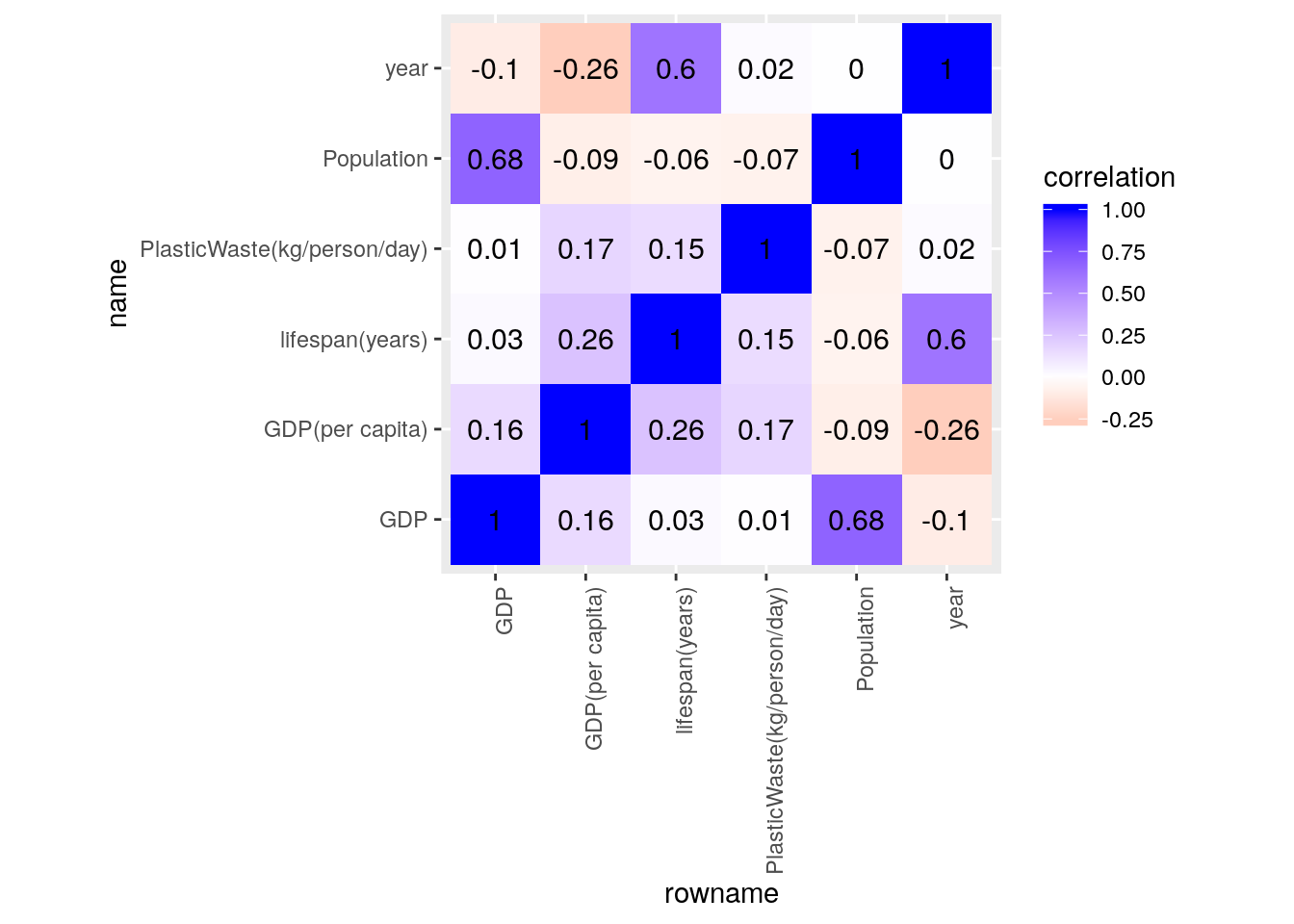
gdpdataplot1 <- gdpdata %>% arrange(desc(`lifespan(years)`)) %>%
    filter(`lifespan(years)` > 82.5)
ggplot(gdpdataplot1, aes(x = country, y = `lifespan(years)`,
    fill = code)) + scale_y_continuous(breaks = c(10, 20, 30,
    40, 50, 60, 70, 80, 90)) + geom_bar(stat = "summary", fun.y = "mean",
    position = "dodge", color = "darkred") + geom_errorbar(stat = "summary",
    width = 0.5) + theme(axis.text.x = element_text(angle = 45,
    hjust = 1), legend.position = "top") + ggtitle("Top eight countries with high life expectancies") +
    ylab("life expectancy in years")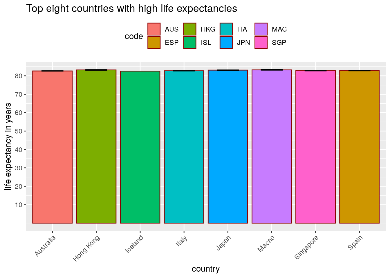
gdpplot2 <- ggplot(data = gdpdataplot1, aes(x = `GDP(per capita)`,
    y = Population, color = country)) + geom_point(size = 2,
    alpha = 0.85)
gdpplot2 + ggtitle("GDP per Capita by Population for top 8 countries with high life expectancy") +
    ylab("GDP per capita in dollars") + xlab("Population") +
    theme_minimal() + scale_y_continuous(breaks = c(2.5e+07,
    5e+07, 1e+08, 1.25e+08))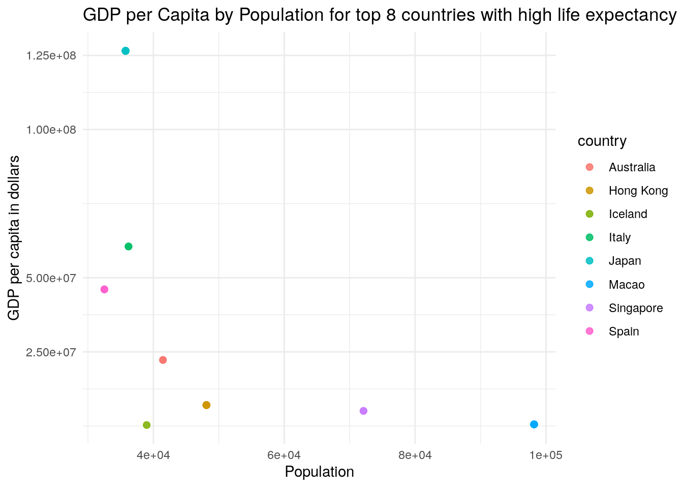
The first plot described the life expectancy in years by country. The box plot clearly showed the top 8 countries with the highest life expectancies (Australia, Hongkong, Iceland, Italy, Japan, Macao, Singapore, and Spain) along with their individual average life expectancies. The color of each of the bars indicates the three letter codes of the country as shown by the legend above the bar plot. The trend that was noticed in this plot was that the top 8 countries with the highest life expectancies all have an average life expectancy a or around 85 years. The tick marks of the bar plot were changed from the default to give a more accurate description of the ages.
The second plot illustrated the GDP per capita by the Population for the top 8 countries with the highest life expectancies. The tick marks of the graph were modified, and the theme was set to a minimal to give a more accurate and clear visualization. The overall trend that was shown to be apparent was that as the population size of the country increases, the GDP per capita of the country drastically decreases.
Dimensionality Reduction
gdpdata2 <- gdpdata %>% select(-"country", -"year", -"PlasticWaste(kg/person/day)",
    -"code", -"GDP", -"Population") %>% glimpse()
## Observations: 10,905
## Variables: 2
## $ `lifespan(years)` <dbl> 54.189, 54.397, 54.872, 55.465, 56.176, 57.003, 57.…
## $ `GDP(per capita)` <dbl> 9927.182, 9927.182, 9927.182, 9927.182, 9927.182, 9…gdpdata3 <- gdpdata %>% select(-"country", -"year", -"code",
-"Population", -"GDP", -"GDP(per capita)") %>% glimpse()## Observations: 10,905
## Variables: 2
## $ `lifespan(years)` <dbl> 54.189, 54.397, 54.872, 55.465, 56.176,…
## $ `PlasticWaste(kg/person/day)` <dbl> 0.069, 0.069, 0.069, 0.069, 0.069, 0.06…gdpdata4 <- gdpdata %>% select(-"country", -"year", -"code",
-"Population", -"GDP", -"lifespan(years)") %>% glimpse()## Observations: 10,905
## Variables: 2
## $ `PlasticWaste(kg/person/day)` <dbl> 0.069, 0.069, 0.069, 0.069, 0.069, 0.06…
## $ `GDP(per capita)` <dbl> 9927.182, 9927.182, 9927.182, 9927.182,…# GDP Per Capita and Life Expectancy
wss <- vector()
for (i in 1:10) {
temp <- gdpdata2 %>% dplyr::select(`lifespan(years)`, `GDP(per capita)`) %>%
kmeans(., i)
wss[i] <- temp$tot.withinss %>% glimpse()
}## num 4.46e+12
## num 1.42e+12
## num 1.1e+12
## num 4.25e+11
## num 3.43e+11
## num 2.89e+11
## num 2.79e+11
## num 2.77e+11
## num 8.77e+10
## num 9.3e+10ggplot() + geom_point(aes(x = 1:10, y = wss)) + geom_path(aes(x = 1:10,
y = wss)) + xlab("clusters") + scale_x_continuous(breaks = 1:10)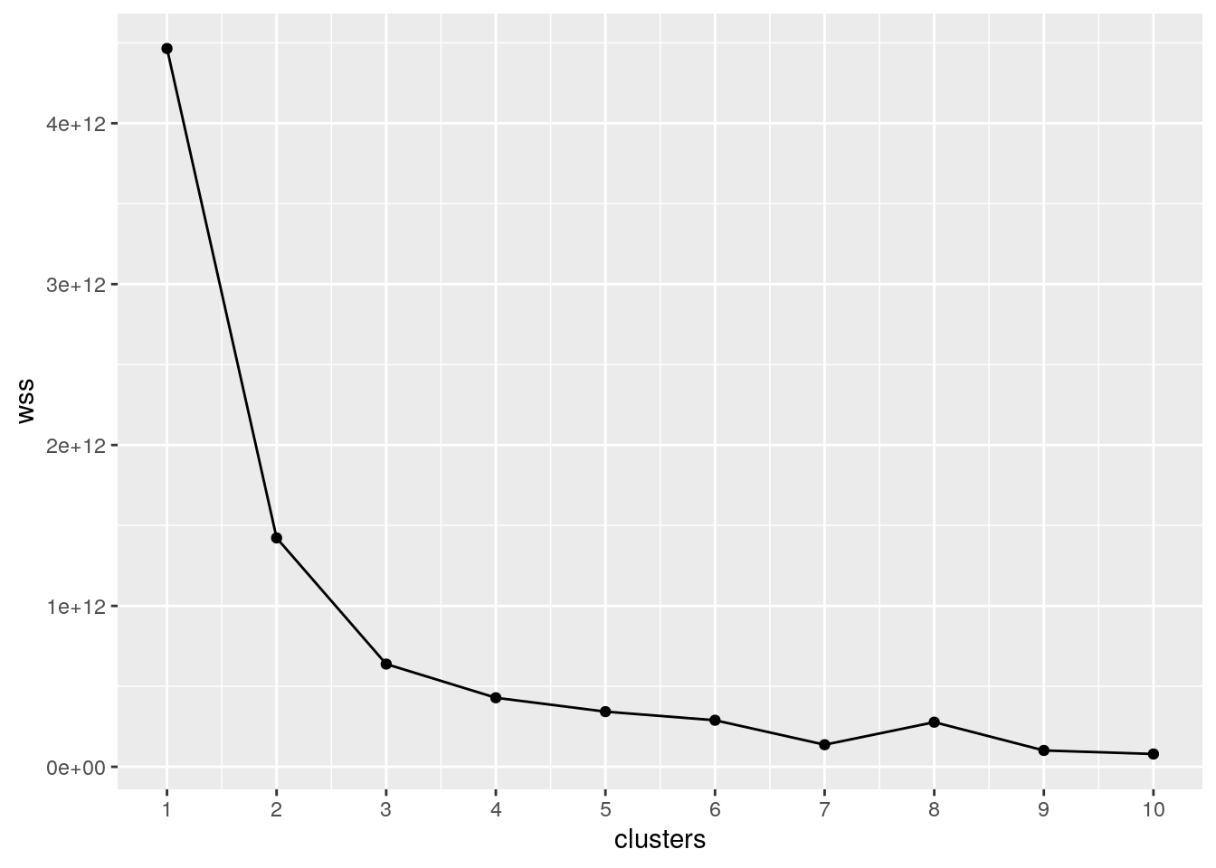
kmeans1 <- kmeans(gdpdata2, 2)
kmeans1
## K-means clustering with 2 clusters of sizes 4085, 6820
##
## Cluster means:
##   lifespan(years) GDP(per capita)
## 1        63.28445       43691.398
## 2        58.43268        9182.814
##
## Clustering vector:
## [1] 2 2 2 2 2 2 2 2 2 2 2 2 2 2 2 2 2 2 2 2 2 2 2 2 2 2 2 2 2 2 2 2 2 2 2 2 2
## [38] 2 2 2 2 2 2 2 2 2 2 2 2 2 2 2 2 2 2 2 2 2 2 2 2 2 2 2 2 2 2 2 2 2 2 2 2 2
## [75] 2 2 2 2 2 2 2 2 2 2 2 2 2 2 2 2 2 2 2 2 2 2 2 2 2 2
## [ reached getOption("max.print") -- omitted 10805 entries ]
##
## Within cluster sum of squares by cluster:
## [1] 1.141688e+12 2.808579e+11
## (between_SS / total_SS = 68.1 %)
##
## Available components:
##
## [1] "cluster" "centers" "totss" "withinss" "tot.withinss"
## [6] "betweenss" "size" "iter" "ifault"kmeanscluster <- gdpdata2 %>% mutate(cluster = as.factor(kmeans1$cluster)) %>%
glimpse## Observations: 10,905
## Variables: 3
## $ `lifespan(years)` <dbl> 54.189, 54.397, 54.872, 55.465, 56.176, 57.003, 57.…
## $ `GDP(per capita)` <dbl> 9927.182, 9927.182, 9927.182, 9927.182, 9927.182, 9…
## $ cluster <fct> 2, 2, 2, 2, 2, 2, 2, 2, 2, 2, 2, 2, 2, 2, 2, 2, 2, …kmeanscluster %>% ggplot(aes(`lifespan(years)`, `GDP(per capita)`,
color = cluster)) + geom_point()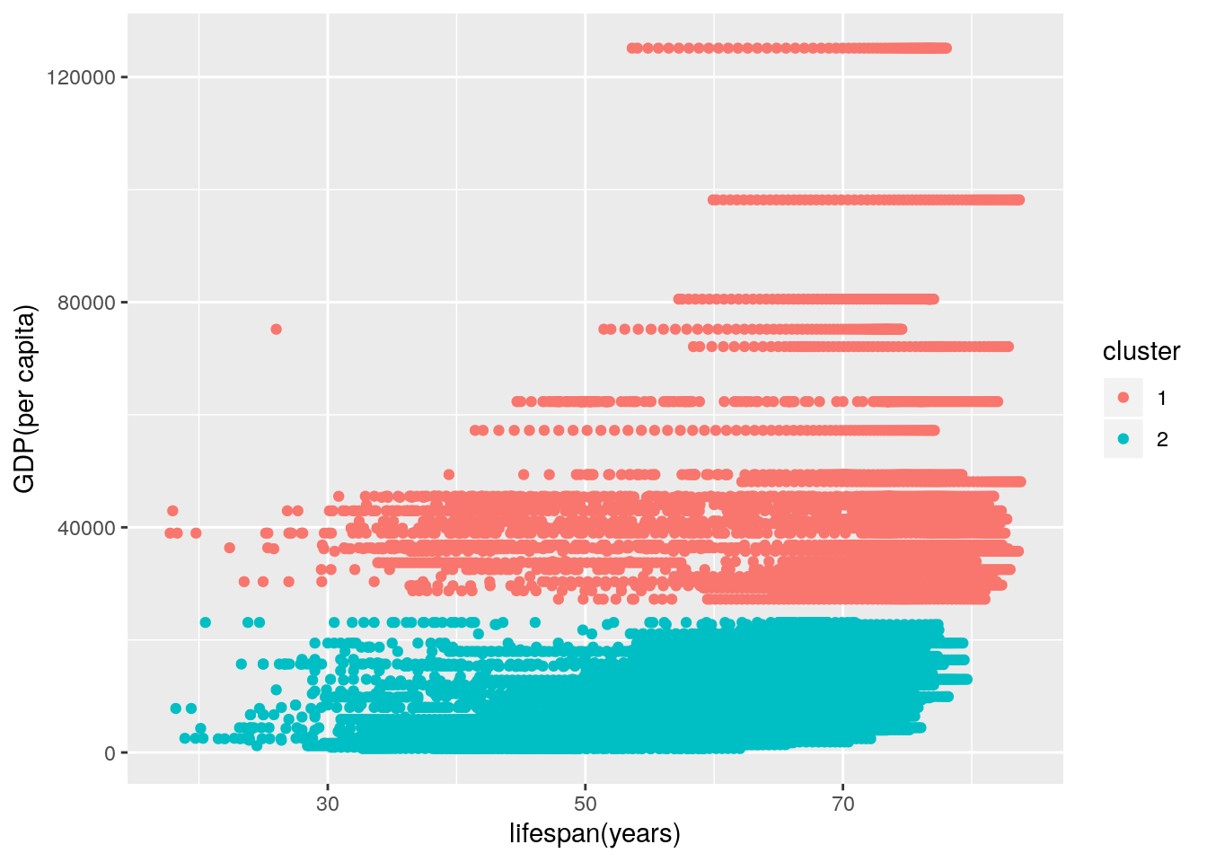
kmeans1$betweenss## [1] 3.042321e+12kmeans1$size## [1] 4085 6820kmeans1$tot.withinss## [1] 1.422546e+12kmeans1$centers## lifespan(years) GDP(per capita)
## 1 63.28445 43691.398
## 2 58.43268 9182.814# Life Expectancy and Plastic Waste
wss2 <- vector()
for (i in 1:10) {
temp3 <- gdpdata3 %>% dplyr::select(`lifespan(years)`, `PlasticWaste(kg/person/day)`) %>%
kmeans(., i)
wss2[i] <- temp3$tot.withinss %>% glimpse()
}## num 1922635
## num 507147
## num 242668
## num 155045
## num 103025
## num 74707
## num 56194
## num 44384
## num 35739
## num 29162ggplot() + geom_point(aes(x = 1:10, y = wss2)) + geom_path(aes(x = 1:10,
y = wss2)) + xlab("clusters") + scale_x_continuous(breaks = 1:10)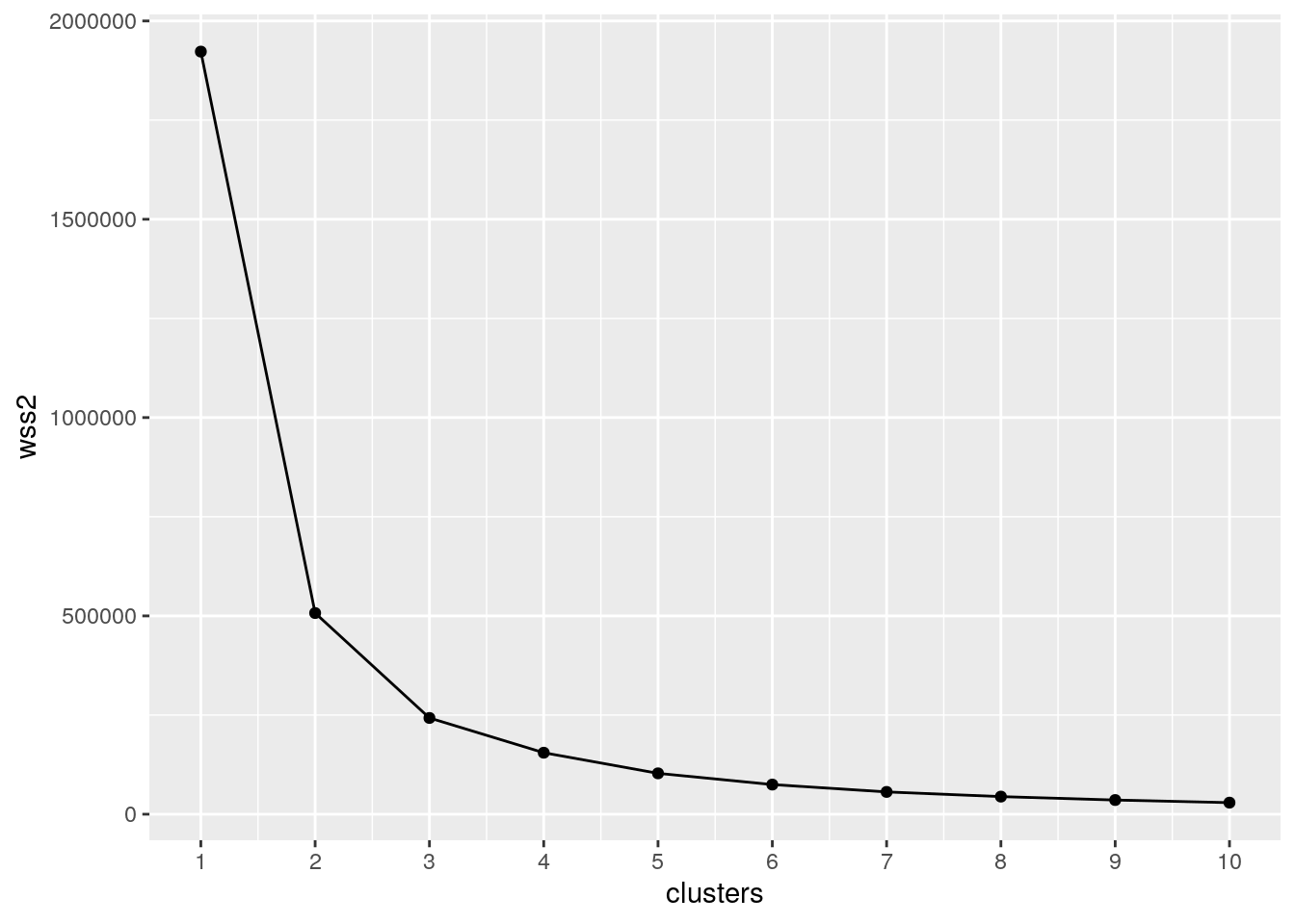
kmeans2 <- kmeans(gdpdata3, 2)
kmeans2
## K-means clustering with 2 clusters of sizes 6650, 4255
##
## Cluster means:
##   lifespan(years) PlasticWaste(kg/person/day)
## 1        69.36344                   0.2319574
## 2        46.00729                   0.1328005
##
## Clustering vector:
## [1] 2 2 2 2 2 2 1 1 1 1 1 1 1 1 1 1 1 1 1 1 1 1 1 1 1 1 1 1 1 1 1 1 1 1 1 1 1
## [38] 1 1 1 1 1 1 1 1 1 1 1 1 1 1 1 1 1 1 1 1 1 1 1 1 1 1 1 1 1 2 2 2 2 2 2 2 2
## [75] 2 2 2 2 2 2 2 2 2 2 2 2 2 2 2 2 2 2 2 2 2 2 2 2 2 1
## [ reached getOption("max.print") -- omitted 10805 entries ]
##
## Within cluster sum of squares by cluster:
## [1] 245337.0 261810.2
## (between_SS / total_SS = 73.6 %)
##
## Available components:
##
## [1] "cluster" "centers" "totss" "withinss" "tot.withinss"
## [6] "betweenss" "size" "iter" "ifault"kmeans2$betweenss## [1] 1415487kmeans2$tot.withinss## [1] 507147.2kmeans2$size## [1] 6650 4255kmeans2$centers## lifespan(years) PlasticWaste(kg/person/day)
## 1 69.36344 0.2319574
## 2 46.00729 0.1328005kmeanscluster2 <- gdpdata3 %>% mutate(cluster = as.factor(kmeans2$cluster)) %>%
glimpse## Observations: 10,905
## Variables: 3
## $ `lifespan(years)` <dbl> 54.189, 54.397, 54.872, 55.465, 56.176,…
## $ `PlasticWaste(kg/person/day)` <dbl> 0.069, 0.069, 0.069, 0.069, 0.069, 0.06…
## $ cluster <fct> 2, 2, 2, 2, 2, 2, 1, 1, 1, 1, 1, 1, 1, …kmeanscluster2 %>% ggplot(aes(`lifespan(years)`, `PlasticWaste(kg/person/day)`,
color = cluster)) + geom_point()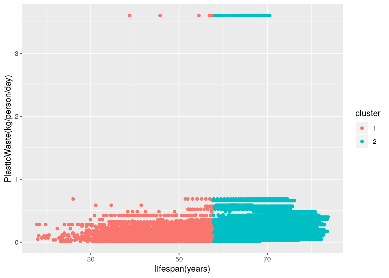
# GDP per capita and Plastic Waste
wss3 <- vector()
for (i in 1:10) {
    temp4 <- gdpdata4 %>% dplyr::select(`GDP(per capita)`, `PlasticWaste(kg/person/day)`) %>%
        kmeans(., i)
    wss3[i] <- temp4$tot.withinss %>% glimpse()
}
## num 4.46e+12
## num 1.42e+12
## num 6.38e+11
## num 4.29e+11
## num 3.43e+11
## num 1.62e+11
## num 2.79e+11
## num 2.66e+11
## num 2.38e+11
## num 2.37e+11ggplot() + geom_point(aes(x = 1:10, y = wss3)) + geom_path(aes(x = 1:10,
y = wss3)) + xlab("clusters") + scale_x_continuous(breaks = 1:10)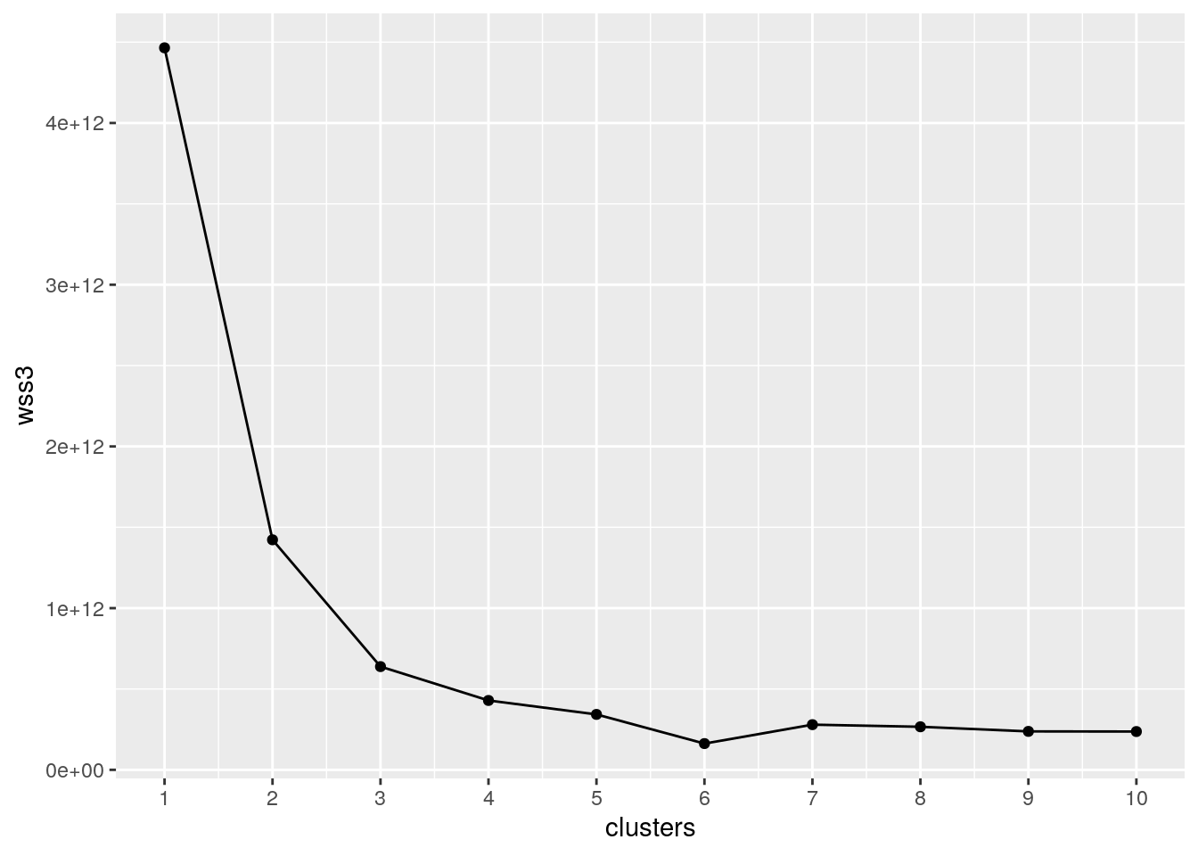
kmeans3 <- kmeans(gdpdata4, 2)
kmeans3
## K-means clustering with 2 clusters of sizes 6820, 4085
##
## Cluster means:
##   PlasticWaste(kg/person/day) GDP(per capita)
## 1                   0.1453893        9182.814
## 2                   0.2732015       43691.398
##
## Clustering vector:
## [1] 1 1 1 1 1 1 1 1 1 1 1 1 1 1 1 1 1 1 1 1 1 1 1 1 1 1 1 1 1 1 1 1 1 1 1 1 1
## [38] 1 1 1 1 1 1 1 1 1 1 1 1 1 1 1 1 1 1 1 1 1 1 1 1 1 1 1 1 1 1 1 1 1 1 1 1 1
## [75] 1 1 1 1 1 1 1 1 1 1 1 1 1 1 1 1 1 1 1 1 1 1 1 1 1 1
## [ reached getOption("max.print") -- omitted 10805 entries ]
##
## Within cluster sum of squares by cluster:
## [1] 2.808569e+11 1.141687e+12
## (between_SS / total_SS = 68.1 %)
##
## Available components:
##
## [1] "cluster" "centers" "totss" "withinss" "tot.withinss"
## [6] "betweenss" "size" "iter" "ifault"kmeans3$tot.withinss## [1] 1.422544e+12kmeans3$centers## PlasticWaste(kg/person/day) GDP(per capita)
## 1 0.1453893 9182.814
## 2 0.2732015 43691.398kmeans3$size## [1] 6820 4085kmeans3$betweenss## [1] 3.042321e+12kmeanscluster3 <- gdpdata4 %>% mutate(cluster = as.factor(kmeans3$cluster))
kmeanscluster3 %>% ggplot(aes(`GDP(per capita)`, `PlasticWaste(kg/person/day)`,
color = cluster)) + geom_point()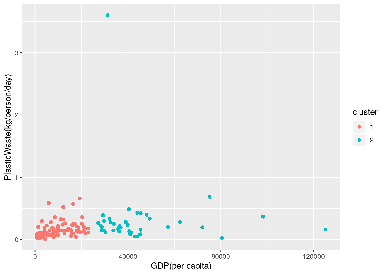
For my data, a k-means cluster for multiple variables was performed on my joined dataset. The first k-means cluster was for GDP per capita and life expectancy. The data was prepped by removing all columns except for the GDP per capita and life expectancy columns. This new dataset was named to be gdpdata2. Next, the number of clusters were determined by the observation of the plot made for clusters vs. wss. The number of clusters were determined by looking at the elbow of the graph that was generated (2 was determined to be the cluster). Next, using k-means cluster, a plot was made using ggplot. Two groups are clearly visible, and from this plot generated it showed that GDP per capita didn’t really show any relationship with life expectancy as countries with low GDP per capita and high GDP per capita all can have high life expectancies. The two clusters were separated by high and low GDp per capita. The betweenss was 3042321025004 and the tot.withinss was 1.422546e+12. The cluster size was 4085 and 6802, with the group having higher GDP per capita containing 6802 countries.
Next, a second k-means cluster for life expectancy and plastic waste was performed. The data was prepped the same way as the first cluster plot generated (dropped all columns except for the columns of interest). The number of clusters to use was determined by the plot of clusters vs wss that was generated. The cluster was again determined to be 2. The cluster was plotted again, and 2 groups were clearly observed. The 2 groups were shown to had been separated based on high and low life expectancy. The two groups were shown to have similar plastic wastes and no relationship was observed between plastic waste and life expectancy. The cluster sizes were 6650 and 4255 with 6650 being cluster 1. In addition, the betweenss was determined to be 1415487 and the tot.withinss was 507147.2.
Lastly, the third k-means cluster was for GDP per capita and plastic waste. The data was prepped the same way as the first two cluster plots generated (dropped all columns except for the columns of interest). The number of clusters was again determined to be 2 by looking at the clusters vs wss plot generated. Then the clusters were plotted, and 2 distinct groups were visualized. The clusters were shown to have been separated based on high and low GDP per capita. There was no clear relationship observed between GDP per capita and plastic waste. The size of the two clusters were 6820 and 4085 with 6820 as cluster 1. The betweenss was 3.042321e+12 and the tot.withinss was 1.422544e+12.